Multiomics data analysis

Cells are the basic functional and structural units of living organisms. They are the location of many different biological processes, which can be probed by various biological techniques. Until recently such data sets have been analysed separately. The aim is to better understand the underlying biological processes and how they influence each other. Therefore techniques that integrate the data from different sources might be applicable [1].

In the image below you see the four main entities that are active throughout the cell: Genome, RNA, proteins, and metabolites. All of them are in constant interaction, for example, some proteins are transcription factors and influence the transcription of DNA into RNA. Metabolites that are present in the cell also influence the activity of proteins as ligands but at the same time are altered through enzymatic activity. This ambiguity of interactions makes it clear that probing the system at a single level gives only limited insight into the structure and function of the cellular processes.


multiomics_schematic

The different levels of biological information (genome, proteome, …) work mutually and influence each other through processes as transcription regulation through transcription factors. All levels are influenced by external factors, as drug treatment or nutrient availability. Multiomics is the measurement of multiple of those populations and their integrated analysis.

In the last years, different ways to integrate such data have been developed. Broadly speaking there are three levels of data integration: conceptual integration, statistical integration, and model-based integration [2]. Conceptual integration means that the data sets are analysed separately and the conclusions are compared and integrated. This method can easily use already existing analysis pipelines but the way in which conclusions are compared and integrated is non-trivial. Statistical Integration combines data sets and analyses them jointly, reaching conclusions that match all data and potentially finding signals that are not observable with the conceptual approach. Model-based integration indicates the joint analysis of the data in a combination of training of a model, which itself might incorporate prior beliefs of a system.

[1] Gehlenborg, Nils, Seán I. O’donoghue, Nitin S. Baliga, Alexander Goesmann, Matthew A. Hibbs, Hiroaki Kitano, Oliver Kohlbacher et al. “Visualization of omics data for systems biology.” Nature methods 7 (2010): S56-S68.

[2] Cavill, Rachel, Danyel Jennen, Jos Kleinjans, and Jacob Jan Briedé. “Transcriptomic and metabolomic data integration.” Briefings in bioinformatics 17, no. 5 (2016): 891-901.

Protein Structure Classification: Order in the Chaos

The number of known protein structures has increased exponentially over the past decades; there are currently over 127,000 structures deposited in the PDB [1]. To bring order to this large volume of data, and to further our understanding of protein function and evolution, these structures are systematically classified according to sequence and structural similarity. Downloadable classification data can be used for annotating datasets, exploring the properties of proteins and for the training and benchmarking of new methods [2].

Yearly growth of structures in the PDB (adapted from [1])

Typically, proteins are grouped by structural similarity and organised using hierarchical clustering. Proteins are sorted into classes based on overall secondary structure composition, and grouped into related families and superfamilies. Although this process could originally be manually curated, as with Structural Classification of Proteins (SCOP) [3] (last updated in June 2009), the growing number of protein structures now requires semi- or fully-automated methods, such as SCOP-extended (SCOPe) [4] and Class, Architecture, Topology, Homology (CATH) [5]. These resources are comprehensive and widely used, particularly in computational protein research. There is a large proportion of agreement between these databases, but subjectivity of protein classification is to be expected. Variation in methods and hierarchical structure result in differences in classifications.  For example, different criteria for defining and classifying domains results in inconsistencies between CATH and SCOPe.

The arrangements of secondary structure elements in space are known as folds. As a result of evolution, the number of folds that exist in nature is thought to be finite, predicted to be between 1000-10,000 [6]. Analysis of currently known structures appears to support this hypothesis, although solved structures in the PDB are likely to be a skewed sample of all protein structures space. Some folds are extremely commonly observed in protein structures.

In his ‘periodic table for protein structures’, William Taylor went one step further in his goal to find a comprehensive, non-hierarchical method of protein classification [7]. He attempted to identify a minimal set of building blocks, referred to as basic Forms, that can be used to assemble as many globular protein structures as possible. These basic Forms can be combined systematically in layers in a way analogous to the combination of electrons into valence shells to form the periodic table. An individual protein structure can then be described as the closest matching combination of these basic Forms.  Related proteins can be identified by the largest combination of basic Forms they have in common.

The ‘basic Forms’ that make up Taylor’s ‘periodic table of proteins’. These secondary structure elements accounted for, on average, 80% of each protein in a set of 2,230 structures (all-alpha proteins were excluded from the dataset) [7]

The classification of proteins by sequence, secondary and tertiary structure is extensive. A relatively new frontier for protein classification is the quaternary structure: how proteins assemble into di-, tri- and multimeric complexes. In a recent publication by an interdisciplinary team of researchers, an analysis of multimeric protein structures in combination with mass spectrometry data was used to create a ‘periodic table of protein complexes’ [8]. Three main types of assembly steps were identified: dimerisation, cyclisation and heteromeric subunit addition. These types are systematically combined to predict many possible topologies of protein complexes, within which the majority of known complexes were found to reside. As has been the case with tertiary structure, this classification and exploration of of quaternary structure space could lead to a better understanding of protein structure, function and evolutionary relationships. In addition, it may inform the modelling and docking of multimeric proteins.


  1. RCSB PDB Statistics
  2. Fox, N.K., Brenner, S.E., Chandonia, J.-M., 2015. The value of protein structure classification information-Surveying the scientific literature. Proteins Struct. Funct. Bioinforma. 83, 2025–2038.
  3. Murzin AG, Brenner SE, Hubbard T, Chothia C., 1995. SCOP: a structural classification of proteins database for the investigation of sequences and structures. J Mol Biol. 247, 536–540.
  4. Fox, N.K., Brenner, S.E., Chandonia, J.-M., 2014. SCOPe: Structural Classification of Proteins–extended, integrating SCOP and ASTRAL data and classification of new structures. Nucleic Acids Res. 42, 304-9.
  5. Dawson NL, Lewis TE, Das S, et al., 2017. CATH: an expanded resource to predict protein function through structure and sequence. Nucleic Acids Research. 45, 289-295.
  6. Derek N Woolfson, Gail J Bartlett, Antony J Burton, Jack W Heal, Ai Niitsu, Andrew R Thomson, Christopher W Wood,. 2015. De novo protein design: how do we expand into the universe of possible protein structures?, Current Opinion in Structural Biology, 33, 16-26.
  7. Taylor, W.R., 2002. A “periodic table” for protein structures. Nature. 416, 657–660.
  8. Ahnert, S.E., Marsh, J.A., Hernandez, H., Robinson, C. V., Teichmann, S.A., 2015. Principles of assembly reveal a periodic table of protein complexes. Science. 80, 350

Prions

The most recent paper presented to the OPIG journal club from PLOS Pathogens, The Structural Architecture of an Infectious Mammalian Prion Using Electron Cryomicroscopy. But prior to that, I presented a bit of a background to prions in general.

In the 1960s, work was being undertaken by Tikvah Alper and John Stanley Griffith on the nature of a transmissible infection which caused scrapie in sheep. They were interested in how studies of the infection showed it was somehow resistant to ionizing radiation. Infectious elements such as bacteria or viruses were normally destroyed by radiation with the amount of radiation required having a relationship with the size of the infectious particle. However, the infection caused by the scrapie agent appeared to be too small to be caused by even a virus.

In 1982, Stanley Prusiner had successfully purified the infectious agent, discovering that it consisted of a protein. “Because the novel properties of the scrapie agent distinguish it from viruses, plasmids, and viroids, a new term “prion” was proposed to denote a small proteinaceous infectious particle which is resistant to inactivation by most procedures that modify nucleic acids.”
Prusiner’s discovery led to him being awarded the Nobel Prize in 1997.

Whilst there are many different forms of infection, such as parasites, bacteria, fungi and viruses, all of these have a genome. Prions on the other hand are just proteins. Coming in two forms, the naturally occurring cellular (PrPC) and the infectious form PrPSC (Sc referring to scrapie), through an as yet unknown mechanism, PrPSC prions are able to reproduce by forcing beneign PrPC forms into the wrong conformation.  It’s believed that through this conformational change, the following diseases are caused.

  • Bovine Spongiform encephalopathy (mad cow disease)
  • Scrapie in:
    • Sheep
    • Goats
  • Chronic wasting disease in:
    • Deer
    • Elk
    • Moose
    • Reindeer
  • Ostrich spongiform encephalopathy
  • Transmissible mink encephalopathy
  • Feline spongiform  encephalopathy
  • Exotic ungulate encephalopathy
    • Nyala
    • Oryx
    • Greater Kudu
  • Creutzfeldt-Jakob disease in humans


Whilst it’s commonly accepted that prions are the cause of the above diseases there’s still debate whether the fibrils which are formed when prions misfold are the cause of the disease or caused by it. Due to the nature of prions, attempting to cure these diseases proves extremely difficult. PrPSC is extremely stable and resistant to denaturation by most chemical and physical agents. “Prions have been shown to retain infectivity even following incineration or after being subjected to high autoclave temperatures“. It is thought that chronic wasting disease is normally transmitted through the saliva and faeces of infected animals, however it has been proposed that grass plants bind, retain, uptake, and transport infectious prions, persisting in the environment and causing animals consuming the plants to become infected.

It’s not all doom and gloom however, lichens may long have had a way to degrade prion fibrils. Not just a way, but because it’s apparently no big thing to them, have done so twice. Tests on three different lichens species: Lobaria pulmonaria, Cladonia rangiferina and Parmelia sulcata, indicated at least two logs of reduction, including reduction “following exposure to freshly-collected P. sulcata or an aqueous extract of the lichen”. This has the potential to inactivate the infectious particles persisting in the landscape or be a source for agents to degrade prions.

Parallel Computing: GNU Parallel

Recently I started using the OPIG servers to run the algorithm I have developed (CRANkS) on datasets from DUDE (Database of Useful Decoys Enhanced).

This required learning how to run jobs in parallel. Previously I had been using computer clusters with their own queuing system (Torque/PBS) which allowed me to submit each molecule to be scored by the algorithm as a separate job. The queuing system would then automatically allocate nodes to jobs and execute jobs accordingly. On a side note I learnt how to submit these jobs an array, which was preferable to submitting ~ 150,000 separate jobs:

qsub -t 1:X array_submit.sh

where the contents of array_submit.sh would be:

#!/bin/bash
./$SGE_TASK_ID.sh

which would submit jobs 1.sh to X.sh, where X is the total number of jobs.

However the OPIG servers do not have a global queuing system to use. I needed a way of being able to run the code I already had in parallel with minimal changes to the workflow or code itself. There are many ways to run jobs in parallel, but to minimise work for myself, I decided to use GNU parallel [1].

This is an easy-to-use shell tool, which I found quick and easy to install onto my home server, allowing me to access it on each of the OPIG servers.

To use it I simply run the command:

cat submit.sh | parallel -j Y

where Y is the number of cores to run the jobs on, and submit.sh contains:

./1.sh
./2.sh
...
./X.sh

This executes each job making use of Y number of cores when available to run the jobs in parallel.

Quick, easy, simple and minimal modifications needed! Thanks to Jin for introducing me to GNU Parallel!

[1] O. Tange (2011): GNU Parallel – The Command-Line Power Tool, The USENIX Magazine, February 2011:42-47.

Interesting Jupyter and IPython Notebooks

Here’s a treasure trove of interesting Jupyter and iPython notebooks, with lots of diverse examples relevant to OPIG, including an RDKit notebook, but also:

Entire books or other large collections of notebooks on a topic (covering Introductory Tutorials; Programming and Computer Science; Statistics, Machine Learning and Data Science; Mathematics, Physics, Chemistry, Biology; Linguistics and Text Mining; Signal Processing; Scientific computing and data analysis with the SciPy Stack; General topics in scientific computing; Machine Learning, Statistics and Probability; Physics, Chemistry and Biology; Data visualization and plotting; Mathematics; Signal, Sound and Image Processing; Natural Language Processing; Pandas for data analysis); General Python Programming; Notebooks in languages other than Python (Julia; Haskell; Ruby; Perl; F#; C#); Miscellaneous topics about doing various things with the Notebook itself; Reproducible academic publications; and lots more!  


Interesting Antibody Papers

Hints how broadly neutralizing antibodies arise (paper here). (Haynes lab here) Antibodies can be developed to bind virtually any antigen. There is a stark difference however between the ‘binding’ antibodies and ‘neutralizing’ antibodies. Binding antibodies are those that make contact with the antigen and perhaps flag it for elimination. This is in contrast to neutralizing antibodies, whose binding eliminates the biological activity of the antigen. A special class of such neutralizing antibodies are ‘broad neutralizing antibodies’. These are molecules which are capable of neutralizing multiple strains of the antigen. Such broadly neutralizing antibodies are very important in the fight against highly malleable diseases such as Influenza or HIV.

The process how such antibodies arise is still poorly understood. In the manuscript of Williams et al., they make a link between the memory and plasma B cells of broadly neutralizing antibodies and find their common ancestor. The common ancestor turned out to be auto-reactive, which might suggest that some degree of tolerance is necessary to allow for broadly neutralizing abs (‘hit a lot of targets fatally’). From a more engineering perspective, they create chimeras of the plasma and memory b cells and demonstrate that they are much more powerful in neutralizing HIV.

Ineresting data: their crystal structures are different broadly neutralizing abs co-crystallized with the same antigen (altought small…). Good set for ab-specific docking or epitope prediction — beyond the other case like that in the PDB (lysozyme)! At the time of writing the structures were still on hold in the PDB so watch this space…

Using RDKit to load ligand SDFs into Pandas DataFrames

If you have downloaded lots of ligand SDF files from the PDB, then a good way of viewing/comparing all their properties would be to load it into a Pandas DataFrame.

RDKit has a very handy function just for this – it’s found under the PandasTool module.

I show an example below within Jupypter-notebook, in which I load in the SDF file, view the table of molecules and perform other RDKit functions to the molecules.

First import the PandasTools module:

from rdkit.Chem import PandasTools

Read in the SDF file:

SDFFile = "./Ligands_noHydrogens_noMissing_59_Instances.sdf"
BRDLigs = PandasTools.LoadSDF(SDFFile)

You can see the whole table by calling the dataframe:

BRDLigs

The ligand properties in the SDF file are stored as columns. You can view what these properties are, and in my case I have loaded 59 ligands each having up to 26 properties:

BRDLigs.info()

It is also very easy to perform other RDKit functions on the dataframe. For instance, I noticed there is no heavy atom column, so I added my own called ‘NumHeavyAtoms’:

BRDLigs['NumHeavyAtoms']=BRDLigs.apply(lambda x: x['ROMol'].GetNumHeavyAtoms(), axis=1)

Here is the column added to the table, alongside columns containing the molecules’ SMILES and RDKit molecule:

BRDLigs[['NumHeavyAtoms','SMILES','ROMol']]

R or Python for data vis?

Python users: ever wanted to learn R?
R users: ever wanted to learn Python?
Check out: http://mathesaurus.sourceforge.net/r-numpy.html

Both languages are incredibly powerful for doing large-scale data analyses. They both have amazing data visualisation platforms, allowing you to make custom graphs very easily (e.g. with your own set of fonts, color palette choices, etc.) These are just a quick run-down of the good, bad, and ugly:

R

  • The good:
    • More established in statistical analyses; if you can’t find an R package for something, chances are it won’t be available in Python either.
    • Data frame parsing is fast and efficient, and incredibly easy to use (e.g. indexing specific rows, which is surprisingly hard in Pandas)
    • If GUIs are your thing, there are programs like Rstudio that mesh the console, plotting, and code.
  • The bad:
    • For loops are traditionally slow, meaning that you have to use lots of apply commands (e.g. tapply, sapply).
  • The ugly:
    • Help documentation can be challenging to read and follow, leading to (potentially) a steep learning curve.

Python

  • The good:
    • If you have existing code in Python (e.g. analysing protein sequences/structures), then you can plot straight away without having to save it as a separate CSV file for analysis, etc.
    • Lots of support for different packages such as NumPy, SciPy, Scikit Learn, etc., with good documentation and lots of help on forums (e.g. Stack Overflow)
    • It’s more useful for string manipulation (e.g. parsing out the ordering of IMGT numbering for antibodies, which goes from 111A->111B->112B->112A->112)
  • The bad:
    • Matplotlib, which is the go-to for data visualisation, has a pretty steep learning curve.
  • The ugly:
    • For statistical analyses, model building can have an unusual syntax. For example, building a linear model in R is incredibly easy (lm), whereas Python involves sklearn.linear_model.LinearRegression().fit. Otherwise you have to code up a lot of things yourself, which might not be practical.

For me, Python wins because I find it’s much easier to create an analysis pipeline where you can go from raw data (e.g. PDB structures) to analysing it (e.g. with BioPython) then plotting custom graphics. Another big selling point is that Python packages have great documentation. Of course, there are libraries to do the analyses in R but the level of freedom, I find, is a bit more restricted, and R’s documentation means you’re often stuck interpreting what the package vignette is saying, rather than doing actual coding.

As for plotting (because pretty graphs are where it’s at!), here’s a very simple implementation of plotting the densities of two normal distributions, along with their means and standard deviations.

import numpy as np
from matplotlib import rcParams

# plt.style.use('xkcd') # A cool feature of matplotlib is stylesheets, e.g. make your plots look XKCD-like

# change font to Arial
# you can change this to any TrueType font that you have in your machine
rcParams['font.family'] = 'sans-serif'
rcParams['font.sans-serif'] = ['Arial']

import matplotlib.pyplot as plt
# Generate two sets of numbers from a normal distribution
# one with mean = 4 sd = 0.5, another with mean (loc) = 1 and sd (scale) = 2
randomSet = np.random.normal(loc = 4, scale = 0.5, size = 1000)
anotherRandom = np.random.normal(loc = 1, scale = 2, size = 1000)

# Define a Figure and Axes object using plt.subplots
# Axes object is where we do the actual plotting (i.e. draw the histogram)
# Figure object is used to configure the actual figure (e.g. the dimensions of the figure)
fig, ax = plt.subplots()

# Plot a histogram with custom-defined bins, with a blue colour, transparency of 0.4
# Plot the density rather than the raw count using normed = True
ax.hist(randomSet, bins = np.arange(-3, 6, 0.5), color = '#134a8e', alpha = 0.4, normed = True)
ax.hist(anotherRandom, bins = np.arange(-3, 6, 0.5), color = '#e8291c', alpha = 0.4, normed = True)

# Plot solid lines for the means
plt.axvline(np.mean(randomSet), color = 'blue')
plt.axvline(np.mean(anotherRandom), color = 'red')

# Plot dotted lines for the std devs
plt.axvline(np.mean(randomSet) - np.std(randomSet), linestyle = '--', color = 'blue')
plt.axvline(np.mean(randomSet) + np.std(randomSet), linestyle = '--', color = 'blue')

plt.axvline(np.mean(anotherRandom) - np.std(anotherRandom), linestyle = '--', color = 'red')
plt.axvline(np.mean(anotherRandom) + np.std(anotherRandom), linestyle = '--', color = 'red')

# Set the title, x- and y-axis labels
plt.title('A fancy plot')
ax.set_xlabel("Value of $x$") 
ax.set_ylabel("Density")

# Set the Figure's size as a 5in x 5in figure
fig.set_size_inches((5,5))

Figure made by matplotlib using the code above.

randomSet = rnorm(mean = 4, sd = 0.5, n = 1000)
anotherRandom = rnorm(mean = 1, sd = 2, n = 1000)

# Let's define a range to plot the histogram for binning;
limits = range(randomSet, anotherRandom)
lbound = limits[1] - (diff(limits) * 0.1)
ubound = limits[2] + (diff(limits) * 0.1)
# use freq = F to plot density
# in breaks, we define the bins of the histogram by providing a vector of values using seq
# xlab, ylab define axis labels; main sets the title
# rgb defines the colour in RGB values from 0-1, with the fourth digit setting transparency
# e.g. rgb(0,1,0,1) is R = 0, G = 1, B = 0, with a alpha of 1 (i.e. not transparent)
hist(randomSet, freq = F, breaks = seq(lbound, ubound, 0.5), col = rgb(0,0,1,0.4), xlab = 'Value of x', ylab = 'Density', main = 'A fancy plot')
# Use add = T to keep both histograms in one graph
# other parameters, such as breaks, etc., can be introduced here
hist(anotherRandom, freq = F, breaks = seq(lbound, ubound, 0.5), col = rgb(1,0,0,0.4), add = T)

# Plot vertical lines with v =
# lty = 2 generates a dashed line
abline(v = c(mean(randomSet), mean(anotherRandom)), col = c('blue', 'red'))

abline(v = c(mean(randomSet)-sd(randomSet), mean(randomSet)+sd(randomSet)), col = 'blue', lty = 2)
abline(v = c(mean(anotherRandom)-sd(anotherRandom), mean(anotherRandom)+sd(anotherRandom)), col = 'red', lty = 2)

Similar figure made using R code from above.

*Special thanks go out to Ali and Lyuba for helpful fixes to make the R code more efficient!

Confidence (scores) in STRING

There are many techniques for inferring protein interactions (be it physical binding or functional associations), and each one has its own quirks: applicability, biases, false positives, false negatives, etc. This means that the protein interaction networks we work with don’t map perfectly to the biological processes they attempt to capture, but are instead noisy observations.

The STRING database tries to quantify this uncertainty by assigning scores to proposed protein interactions based on the nature and quality of the supporting evidence. STRING contains functional protein associations derived from in-house predictions and homology transfers, as well as taken from a number of externally maintained databases. Each of these interactions is assigned a score between zero and one, which is (meant to be) the probability that the interaction really exists given the available evidence.

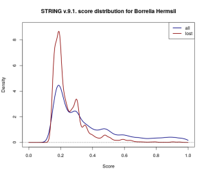
Throughout my short research project with OPIG last year I worked with STRING data for Borrelia Hermsii, a relatively small network of scored interactions across 815 proteins. I was working with v.10.0., the latest available database release, but also had the chance to compare this to v.9.1 data. I expected that with data from new experiments and improved scoring methodologies available, the more recent network would be more or less a re-scored superset of the older. Even if some low-scored interactions weren’t carried across the update, I didn’t expect these to be any significant proportion of the data. Interestingly enough, this was not the case.

Out of 31 264 scored protein-protein interactions in v.9.1. there were 10 478, i.e. almost exactly a third of the whole dataset, which didn’t make it across the update to v.10.0. The lost interactions don’t seem to have very much in common either — they come from a range of data sources and don’t appear to be located within the same region of the network. The update also includes 21 192 previously unrecorded interactions.

densityComparison

Gaussian kernel density estimates for the score distribution of interactions across the entire 9.1. Borrelia Hermsii dataset (navy) and across the discarded proportion of the dataset (dark red). Proportionally more low-scored interactions have been discarded.

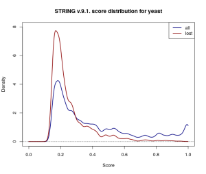
Repeating the comparison with baker’s yeast (Saccharomyces cerevisiae), a much more extensively studied organism, shows this isn’t a one-off case either. The yeast network is much larger (777 589 scored interactions across 6400 proteins in STRING v.9.1.), and the changes introduced by v.10.0. appear to be scaled accordingly — 237 427 yeast interactions were omitted in the update, and 399 836 new ones were added.

discardedYeast

Kernel density estimates for the score distribution for yeast in STRING v.9.1. While the overall (navy) and discarded (dark red) score distributions differ from the ones for Borrelia Hermsii above, a similar trend of omitting more low-scored edges is observed.

So what causes over 30% of the scored interactions in the database to disappear into thin air? At least in part this may have to do with thresholding and small changes to the scoring procedure. STRING truncates reported interactions to those with a score above 0.15. Estimating how many low-scored interactions have been lost from the original dataset in this way is difficult, but the wide coverage of gene co-expression data would suggest that they’re a far from negligible proportion of the scored networks. The changes to the co-expression scoring pipeline in the latest release [1], coupled with the relative abundance of co-expression data, could have easily shifted scores close to 0.15 on the other side of the threshold, and therefore might explain some of the dramatic difference.

However, this still doesn’t account for changes introduced in other channels, or for interactions which have non-overlapping types of supporting evidence recorded in the two database versions. Moreover, thresholding at 0.15 adds a layer of uncertainty to the dataset — there is no way to distinguish between interactions where there is very weak evidence (i.e. score below 0.15), pairs of proteins that can be safely assumed not to interact (i.e. a “true” score of 0), and pairs of proteins for which there is simply no data available. While very weak evidence might not be of much use when studying a small part of the network, it may have consequences on a larger scale: even if only a very small fraction of these interactions are true, they might be indicative of robustness in the network, which can’t be otherwise detected.

In conclusion, STRING is a valuable resource of protein interaction data but one ought to take the reported scores with a grain of salt if one is to take a stochastic approach to protein interaction networks. Perhaps if scoring pipelines were documented in a way that made them reproducible and if the data wasn’t thresholded, we would be able to study the uncertainty in protein interaction networks with a bit more confidence.

References:

[1] Szklarczyk, Damian, et al. “STRING v10: protein–protein interaction networks, integrated over the tree of life.” Nucleic acids research (2014): gku1003

Interesting Antibody Papers

Below are two somewhat recent papers that are quite relevant to those doing ab-engineering. The first one takes a look at antibodies as a collection — software which better estimates a diversity of an antibody repertoire. The second one looks at each residue in more detail — it maps the mutational landscape of an entire antibody, showing a possible modulating switch for VL-CL interface.

Estimating the diversity of an antibody repertoire. (Arnaout Lab) paper here. High Throughput Sequencing (or next generation sequencing…) of antibody repertoires allows us to get snapshots of the overall antibody population. Since the antibody population ‘diversity’ is key to their ability to find a binder to virtually any antigen, it is desirable to quantify how ‘diverse’ the sample is as a way to see how broad you need to cast the net. Firstly however, we need to know what we mean by ‘diversity’. One way of looking at it is akin to considering ‘species diversity’, studied extensively in ecology. For example, you estimate the ‘richness’ of species in a sample of 100 rabbits, 10 wolves and 20 sheep. Diversity measures such as Simpson’s index or entropy were used to calculate how biased the diversity is towards one species. Here the sample is quite biased towards rabbits, however if instead we had 10 rabbits, 10 wolves and 10 sheep, the ‘diversity’ would be quite uniform. Back to antibodies: it is desirable to know if a given species of an antibody is more represented than others or if one is very underrepresented. This might indicate healthy vs unhealthy immune system, indicate antibodies carrying out an immune response (when there is more of a type of antibody which is directing the immune response). Problem: in an arbitrary sample of antibody sequences/reads tell me how diverse they are. We should be able to do this by estimating the number of cell clones that gave rise to the antibodies (referred to as clonality). People have been doing this by grouping sequences by CDR3 similarity. For example, sequences with CDR3 identical or more than >95% identity, are treated as the same cell — which is tantamount to being the same ‘species’. However since the number of diverse B cells in a human organism is huge, HTS only provides a sample of these. Therefore some rarer clones might be underrepresented or missing altogether. To address this issue, Arnaout and Kaplinsky developed a methodology called Recon which estimates the antibody sample diversity. It is based on the expectation-maximization algorithm: given a list of species and their numbers, iterate adding parameters until they have a good agreement between the fitted distributions and the given data. They have validated this methodology firstly on the simulated data and then on the DeKosky dataset. The code is available from here subject to their license agreement.

Thorough analysis of the mutational landscape of the entire antibody. [here]. (Germaine Fuh from Affinta/Genentech/Roche). The authors aimed to see how malleable the variable antibody domains are to mutations by introducing all possible modifications at each site in an example antibody. As the subject molecule they have used high-affinity, very stable anti-VEGF antibody G6.31. They argue that this antibody is a good representative of human antibodies (commonly used genes Vh3, Vk1) and that its optimized CDRs might indicate well any beneficial distal mutations. They confirm that the positions most resistant to mutation are the core ones responsible for maintaining the structure of the molecule. Most notably here, they have identified that Kabat L83 position correlates with VL-CL packing. This position is most frequently a phenylalanine and less frequently valine or alanine. This residue is usually spatially close to isoleucine at position LC-106. They have defined two conformations of L83F — in and out:

  1. Out: -50<X1-100 interface.
  2. In: 50<X1<180

Being in either of these positions correlates with the orientation of LC-106 in the elbow region. This in turn affects how big the VL-CL interface is (large elbow angle=small  tight interface; small elbow angle=large interface). The L83 position often undergoes somatic hypermutation, as does the LC-106 with the most common mutation being valine.