Below are two somewhat recent papers that are quite relevant to those doing ab-engineering. The first one takes a look at antibodies as a collection — software which better estimates a diversity of an antibody repertoire. The second one looks at each residue in more detail — it maps the mutational landscape of an entire antibody, showing a possible modulating switch for VL-CL interface.

Estimating the diversity of an antibody repertoire. (Arnaout Lab) paper here. High Throughput Sequencing (or next generation sequencing…) of antibody repertoires allows us to get snapshots of the overall antibody population. Since the antibody population ‘diversity’ is key to their ability to find a binder to virtually any antigen, it is desirable to quantify how ‘diverse’ the sample is as a way to see how broad you need to cast the net. Firstly however, we need to know what we mean by ‘diversity’. One way of looking at it is akin to considering ‘species diversity’, studied extensively in ecology. For example, you estimate the ‘richness’ of species in a sample of 100 rabbits, 10 wolves and 20 sheep. Diversity measures such as Simpson’s index or entropy were used to calculate how biased the diversity is towards one species. Here the sample is quite biased towards rabbits, however if instead we had 10 rabbits, 10 wolves and 10 sheep, the ‘diversity’ would be quite uniform. Back to antibodies: it is desirable to know if a given species of an antibody is more represented than others or if one is very underrepresented. This might indicate healthy vs unhealthy immune system, indicate antibodies carrying out an immune response (when there is more of a type of antibody which is directing the immune response). Problem: in an arbitrary sample of antibody sequences/reads tell me how diverse they are. We should be able to do this by estimating the number of cell clones that gave rise to the antibodies (referred to as clonality). People have been doing this by grouping sequences by CDR3 similarity. For example, sequences with CDR3 identical or more than >95% identity, are treated as the same cell — which is tantamount to being the same ‘species’. However since the number of diverse B cells in a human organism is huge, HTS only provides a sample of these. Therefore some rarer clones might be underrepresented or missing altogether. To address this issue, Arnaout and Kaplinsky developed a methodology called Recon which estimates the antibody sample diversity. It is based on the expectation-maximization algorithm: given a list of species and their numbers, iterate adding parameters until they have a good agreement between the fitted distributions and the given data. They have validated this methodology firstly on the simulated data and then on the DeKosky dataset. The code is available from here subject to their license agreement.

Thorough analysis of the mutational landscape of the entire antibody. [here]. (Germaine Fuh from Affinta/Genentech/Roche). The authors aimed to see how malleable the variable antibody domains are to mutations by introducing all possible modifications at each site in an example antibody. As the subject molecule they have used high-affinity, very stable anti-VEGF antibody G6.31. They argue that this antibody is a good representative of human antibodies (commonly used genes Vh3, Vk1) and that its optimized CDRs might indicate well any beneficial distal mutations. They confirm that the positions most resistant to mutation are the core ones responsible for maintaining the structure of the molecule. Most notably here, they have identified that Kabat L83 position correlates with VL-CL packing. This position is most frequently a phenylalanine and less frequently valine or alanine. This residue is usually spatially close to isoleucine at position LC-106. They have defined two conformations of L83F — in and out:

1. Out: -50<X1-100 interface.
2. In: 50<X1<180

Being in either of these positions correlates with the orientation of LC-106 in the elbow region. This in turn affects how big the VL-CL interface is (large elbow angle=small  tight interface; small elbow angle=large interface). The L83 position often undergoes somatic hypermutation, as does the LC-106 with the most common mutation being valine.

At the meeting on November 15 I have covered a paper by Gantz et al. describing a method for creating transgenic mosquitoes expressing antibodies hindering the development of malaria parasites.

The immune system is commonly divided into two categories: innate and adaptive. The innate immune system consists of non-specific defence mechanisms such as epithelial barriers, macrophages etc. The innate system is present in virtually every living organism. The adaptive immune system is responsible for invader-specific defence response. Is consists of B and T lymphocytes and encompasses antibody production. As only vertebrates posses the adaptive immune system, mosquitoes do not naturally produce antibodies which hinders their ability to defend themselves against pathogens such as malaria.

In the study by Gantz et al. the authors inserted transgenes expressing three single-chain Fvs (m4B7, m2A10 and m1C3) into the previously-characterised chromosomal docking sites.

Figure 1: The RT-PCR experiments showing the scFv expression in different mosquito strains

RT-PCR was used to detect scFv transcripts in RNA isolated from the transgenic mosquitoes (see Figure 1). The experiments showed that the attP 44-C recipient line allowed expression of the transgenes coding for the scFvs.

The authors evaluated the impact of the modifications on the fitness of the mosquitoes. It was shown that the transgene expression does not reduce the lifespan of the mosquitoes, or their ability to procreate.

Expression of the scFvs targeted the parasite at both the early and late development stages. The transgenic mosquitoes displayed a significant reduction in the number of malaria sporozoites per infected female, in most cases completely inhibiting the sporozoite development.

Overall the study showed that it is possible to develop transgenic mosquitoes that are resistant to malaria. If this method was combined with a mechanism for a gene spread, the malaria-resistant mosquitoes could be released into the environment, helping to fight the spread of this disease.

The Era of Crystallography ends…

For over 100 years, crystallography has been used to determine the atom arrangements of molecules; specifically, it has become the workhorse of routine macromolecular structure solution, being responsible for over 90% of the atomic structures in the PDB. Whilst this achievement is impressive, in some ways it has come around despite the crystallographic method, rather than because of it…

The problem, generally, is this: to perform crystallography, you need crystals. Crystals require the spontaneous assembly of billions of molecules into a regular repeated arrangement. For proteins — large, complex, irregularly shaped molecules — this is not generally a natural state for them to exist in, and getting a protein to crystallise can be a difficult process (the notable exception is Lysozyme, which it is difficult NOT to crystallise, and there are subsequently currently ~1700 crystal structures of it in the PDB). Determining the conditions under which proteins will crystallise requires extensive screening: placing the protein into a variety of difference solutions, in the hope that in one of these, the protein will spontaneously self-assemble into (robust, homogeneous) crystals. As for membrane proteins, which… exist in membranes, crystallisation solutions are sort of ridiculous (clever, but ridiculous).

But even once a crystal is obtained (and assuming it is a “good” well-diffracting crystal), diffraction experiments alone are generally not enough to determine the atomic structure of the crystal. In a crystallographic experiment, only half of the data required to solve the structure of the crystal is measured — the amplitudes. The other half of the data — the phases — are not measured. This constitutes the “phase problem” of crystallography, and “causes some problems”: developing methods to solve the phase problem is essentially a field of its own.

…and the Era of Cryo-Electron Microscopy begins

Cryo-electron microscopy (cryo-EM; primers here and here), circumnavigates both of the problems with crystallography described above (although of course it has some of its own). Single-particles of the protein (or protein complex) are deposited onto grids and immobilised, removing the need for crystals altogether. Furthermore, the phases can be measured directly, removing the need to overcome the phase problem.

Cryo-EM is also really good for determining the structures of large complexes, which are normally out of the reach of crystallography, and although cryo-EM structures used to only be determined at low resolution, this is changing quickly with improved experimental hardware.

Cryo-Electron Microscopy is getting better and better every day. For structural biologists, it seems like it’s going to be difficult to avoid it. However, for crystallographers, don’t worry, there is hope.

Last week during the group meeting we talked about a pre-print publication from the Ippolito group in Austin TX (here). The authors were monitoring the antibody repertoire from Bone Marrow Plasma Cells (80% of circulating abs) over a period of 6.5 years. For comparison they have monitored another individual over the period of 2.3 years. In a nutshell, the paper is like Picture 1 — just with antibodies

This is what the paper talks about in a nutshell. How the antibody repertoire looks like taken at different timepoints in an individual’s lifetime.

.

The main question that they aimed to answer was: ‘Is the Human Antibody repertoire stable over time‘? It is plausible to think that there should be some ‘ground distribution’ of antibodies that are present over time which act as a default safety net. However we know that the antibody makeup can change radically especially when challenged by antigen. Therefore, it is interesting to ask, does the immune repertoire maintain a fairly stable distribution or not?

Firstly, it is necessary to define what we consider a stable distribution of the human antibody repertoire. The antibodies undergo the VDJ recombination as well as Somatic Hypermutation, meaning that the >10^10 estimated antibodies that a human is capable of producing have a very wide possible variation. In this publication the authors mostly focused on addressing this question by looking at how the usage of possible V, D and J genes and their combinations changes over time.

Seven snapshots of the immune repertoire were taken from the individual monitored over 6.5 years and two from the individual monitored over 2.3 years. Looking at the usage of the V, D and J genes over time, it appears that the proportion in each of the seven time points appears quite stable (Pic 2). Authors claim similar result looking at the combinations.  This would suggest that our antibody repertoire is biased to sample ‘similar’ antibodies over time. These frequencies were compared to the individual who was sampled over the period of 2.3 years and it appears that the differences might not be great between the two.

How the frequencies of V, D and J genes change (not) over 6.5 years in a single individual

It is a very interesting study which hints that we (humans) might be sampling the antibodies from a biased distribution — meaning that our bodies might have developed a well-defined safety net which is capable of raising an antibody towards an arbitrary antigen. It is an interesting starting point and to further check this hypothesis, it would be necessary to carry out such a study on multiple individuals (as a minimum to see if there are really no differences between us — which would at the same time hint that the repertoire do not change over time).

On the theme of my research area and my last presentation I talked at group meeting about a another success story in structurally designing an antibody by replicating a general protein binding site using grafted fragments involved in the original complex. The paper by Liu et al is important to me for two major reasons . Firstly they used an unconventional antibody for protein design, namely a bovine antibody which is known to have an extended CDR H3. Secondly the fragment was not grafted at the anchor points of the CDR loop.

SFTI-1 is a cyclic peptide and a known trypsin inhibitor. It’s structure is stabilised by a disulphide bridge. The bovine antibody is known to have an extended H3 loop which is essentially a long beta strand stalk with a knob domain at the end. Liu et al removed the knob domain and a portion of the B strand and grafted the acyclic version of the SFTI-1 to it. As I said above this result is very important because it shows we can graft a fragment/loop at places different then the anchor points of the CDR. This opens up the possibility for more diverse fragments to be grafted because of new anchor points,  and also because the fragment will sit further away from the other CDRs and the framework allowing more conformational space. To see how the designed antibody compares to the original peptide they measured the Kd and found a 4 fold increase (9.57 vs 13.3). They hypothesise that this is probably due to the fact that the extended beta strand on the antibody keeps the acyclic SFTI-1 peptide in a more stable conformation.

The problem with the bovine antibody is that if inserted in a human subject it would probably elicit an immune response from the native immune system. To humanise this antibody they found the human framework which shares the greatest sequence identity to the bovine antibody and then grafted the fragment on it. The human antibody does not have an extended CDR H3 and to decide what is the best place of grafting they tried various combinations again showing again that the fragments do not need to grafted exactly at the anchor points. Some of the resulting  human antibodies showed even more impressive Kds.

The best designed human antibody had a 0.79nM Kd, another 10-fold gain . Liu et al hypothesised that this might be due to the fact that the cognate protein forms contacts with residues on the other CDRs even though there is no crystal structure to show this. In order to test this hypothesis they mutated surface residues on the H2 and L1 loop to Alanine which resulted in a 6.7 fold decrease in affinity. The only comment I would have to this is that the mutations to the other CDRs might have destabilized the other CDRs on the antibody which could be the reason for the decrease in affinity.

Experimental errors are common at the moment of generating new data. Often this type of errors are simply due to the inability of the instrument to make precise measurements. In addition, different instruments can have different levels of precision, even-thought they are used to perform the same measurement. Take for example two balances and an object with a mass of 1kg. The first balance, when measuring this object different times might record values of 1.0083 and 1.0091, and the second balance might give values of 1.1074 and 0.9828. In this case the first balance has a higher precision as the difference between its measurements is smaller than the difference between the measurements of balance two.

In order to have some control over this error introduced by the level of precision of the different instruments, they are labelled with a measure of their precision or equivalently with their dispersion .

Let’s assume that the type of information these instruments record is of the form ,  where is an error term, its the value recorded by instrument and where is the fixed true quantity of interest the instrument  is trying to measure. But, what if is not a fixed quantity? or what if the underlying phenomenon that is being measured is also stochastic like the measurement . For example if we are measuring the weight of cattle at different times, or the length of a bacterial cell, or concentration of a given drug in an organism, in addition to the error that arises from the instruments; there is also some noise introduced by dynamical changes of the object that is being measured. In this scenario, the phenomenon of interest, can be given  by a random variable . Therefore the instruments would record quantities of the form .

Under this case, estimating the value of , the expected state of the phenomenon of interest is not a big challenge. Assume that there are values observed from realisations of the variables , which came from different instruments. Here is still a good estimation of as .  Now, a more challenging problem is to infer what is the underlying variability of the phenomenon of interest . Under our previous setup, the problem is reduced to estimating  as we are assuming  and that the instruments record values of the from .

To estimate a standard maximum likelihood approach could be used, by considering the likelihood function:

,

from which the maximum likelihood estimator of is given by the solution to

.

Another more naive approach could use the following result

from which .

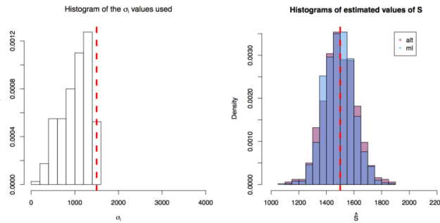
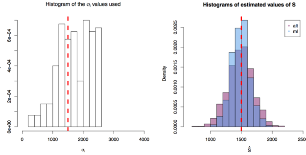
Here are three simulation scenarios where 200 values are taken from instruments of varying precision or variance  and where the variance of the phenomenon of interest . In the first scenario are drawn from , in the second from  and in the third from . In each scenario the value of is estimated 1000 times taking each time another 200 realisations of . The values estimated via the maximum likelihood approach are plotted in blue, and the values obtained by the alternative method are plotted in red. The true value of the is given by the red dashed line across all plots.

First simulation scenario where in . The values of   plotted in the histogram to the right. The 1000 estimations of are shown by the blue (maximum likelihood) and red (alternative) histograms.

First simulation scenario where in . The values of plotted in the histogram to the right. The 1000 estimations of are shown by the blue (maximum likelihood) and red (alternative) histograms.

First simulation scenario where in . The values of plotted in the histogram to the right. The 1000 estimations of are shown by the blue (maximum likelihood) and red (alternative) histograms.

For recent advances in methods that deal with this kind of problems, you can look at:

Something many structural biologists (including us here in OPIG!) are guilty of is treating proteins as static, rigid structures. In reality, proteins are dynamic molecules, transitioning constantly from  conformation to conformation. Proteins are therefore more accurately represented by an ensemble of structures instead of just one.

In my research, I focus on loop structures, the regions of a protein that connect elements of secondary structure (α-helices and β-sheets). There are many examples in the PDB of proteins with identical sequences, but whose loops have different structures. In many cases, a protein’s function depends on the ability of its loops to adopt different conformations. For example, triosephosphate isomerase, which is an important enzyme in the glycolysis pathway, changes conformation upon ligand binding, shielding the active site from solvent and stabilising the intermediate compound so that catalysis can occur efficiently. Conformational variability helps triosephosphate isomerase to be what is known as a ‘perfect enzyme’; catalysis is limited only by the diffusion rate of the substrate.

Structure of the triosephosphate isomerase enzyme. When the substrate binds, a loop changes from an ‘open’ conformation (pink, PDB entry 1TPD) to a ‘closed’ one (green, 1TRD), which prevents solvent access to the active site and stabilises the intermediate compound of the reaction.

An interesting example, especially for some of us here at OPIG, is the antibody SPE7. SPE7 is multispecific, meaning it is able to bind to multiple unrelated antigens. It achieves this through conformational diversity. Four binding site conformations have been found, two of which can be observed in its unbound state in equilibrium – one with a flat binding site, and another with a deep, narrow binding site [1].

SPE7; an antibody that exists as two different structures in equilibrium – one with a shallow binding site (left, blue, PDB code 1OAQ) and one with a deep, narrow cleft (right, green, PDB 1OCW). Complementary determining regions are coloured in each case.

So when you’re dealing with crystal structures, beware! X-ray structures are averages – each atom position is an average of its position across all unit cells. In addition, thanks to factors such as crystal packing, the conformation that we see may not be representative of the protein in solution. The examples above demonstrate that the sequence/structure relationship is not as clear cut as we are often lead to believe. It is important to consider dynamics and conformational diversity, which may be required for protein function. Always bear in mind that the static appearance of an X-ray structure is not the reality!

[1] James, L C, Roversi, P and Tawfik, D S. Antibody Multispecificity Mediated by Conformational Diversity. Science (2003), 299, 1362-1367.

Allosteric (allo-(“other”) + steric (repulsion of atoms due to closeness or arrangement)) sites regulate protein function from a position other than the active site or binding site. Consider the latch on a pair of gardening scissors (Figure 1): depending on the position of the latch (allosteric site) the blades are prevented from cutting things at the other end (active site).

Figure 1 Allostery explained: A safety latch in gardening scissors.

Due to the non-trivial positions of allosteric sites in proteins their identification has been challenging. Selected well characterised systems such as GPCRs have known allosteric sites that are being used as targets in drug development. However, large scale identification of allosteric sites across the Protein Data Base (PDB) has not yet been feasible, partly because of the lack of tools.

To tackle this problem the Gerstein Lab developed a computational protocol based on various molecular simulations and network methods to find allosteric hotspots in proteins across the PDB. They introduce two different pipelines; one for identifying allosteric residues on the surface (surface-critical) and one for buried residues (interior-critical).

For the search of exterior-critical residues they us MC simulations to repeatedly probe the surface of the protein with short Monte Carlo (MC) with a short peptide. Based on hard spheres and simple energy calculations this method seems to be an efficient way of detecting possible binding pockets. Once the binding pockets have been found, the collective motions of the structure are simulated using an elastic mass-and-spring network (an anisotropic network model [ANM]). Binding pockets that undergo significant deformation during these simulations are considered to be surface-critical.

For interior-critical residues they start by weighting residue-residue contacts on the basis of collective movement. Communities within the weighted network are then identified and the residues with the highest betweenness interactions between communities are chosen as interior-critical residues. Thus, interior-critical residues have the highest information flow between two densely inter-connected groups of residues.

The protocol as been implemented in STRESS (STRucturally identified ESSential residues) and is freely available at stress.molmovdb.org.

Publication: http://www.ncbi.nlm.nih.gov/pubmed/27066750

Here’s a little quick round-up of some of the tools/algorithms that I’ve seen in VIZBI, which I believe can be useful for many. For more details, I strongly advise you check out the posters page (vizbi.org/Posters/2016). There were a few that I would’ve liked to re-visit, but the webapps weren’t available (e.g. MeshCloud from the Human Genome Center, Tokyo), so maybe I’ll come back with a part 3. Here are my top five:

1. Autodesk’s Protein Viewer* (shout-outs to @_merrywang on Twitter)
As a structural bioinformatician, I’m going to be really biased here, and say that Autodesk’s Molecule viewer was the best tool that was showcased in the conference. It combines not only the capacity to visualise millions of molecules from the PDB (or your own PDB files), it also allows annotation and sharing, effectively, “snapshots” of your workspace for collaboration (see this if you want to know what I mean). AND it’s free! It’s not the fastest viewer on the planet, nor the easiest thing to use, but it is effective.

2. Vectorbase
Not related to protein structures, but a really interesting visualisation that shows information on, for example, insecticide resistance. With mosquitoes being such a huge part of today’s news, this kind of information is vital for fighting and understanding the distribution of insects across the globe.

3. Phandango
This is a genome browser which, from a one-man effort, could be a game-changer. The UI needs a little bit of work I think, but otherwise, a really valuable tool for crunching lots of genomic data in a quick fashion.

4. i-PV Circos
This is a neat circular browser that helps users view protein sequences in a circularised format. With this visualisation format becoming more popular as the days go by, I think this has the potential to be a leader in the field. At the moment the website’s a bit dark and not the most user-friendly, but some of the core functionality (e.g. highlighting residues and association of domains) is a real plus!

5. Storyline visualisation
Possibly my favourite/eye-opener tool from the entire conference. Storyline visualisation helps users understand how things progress in realtime — this has been used for movie plot data (e.g. Star Wars character and plot progression) but the general concept can be useful for biological phenomena – for example, how do cells in diseased states progress over time? How does it compare to healthy states? Can we also monitor protein dynamics using a similar concept? I think the fact that it gives a very intuitive, big-picture overview of the micro-scale dynamics was the reason why I’ve been incredibly interested in Kwan-Liu Ma’s work, and I recommend checking out his website/publications list to grab insight on improving data visualisation (in particular, network visualisation when you want to avoid hairballs!)

The list isn’t ranked in any way, and do check these out! There were other tools I would’ve really liked to review (e.g. Minardo, made by David Ma @frostickle on Twitter), but I suppose I can go on and on. At the end of the day, visualisation tools like these are meant to be quick, and help us to not only EXPLORE our data, but to EXPLAIN it too. I think we’re incredibly fortunate to have some amazing minds out there who are willing to not only create these tools, but also make them available for all.